Largest $M-1$ values of a set of $N$ independent RVs with different distributions, and sum of remainder, and indexes (exp_ord_spect.m).

We extend the above results to the case when each of the $N$ input RVs have a different distribution $p_i(x_i), \; 1\leq i \leq N$. We restrict the analysis, however, to the case when $t_i = i, \; 1\leq i \leq M-1$ (the largest $M-1$ RV). We would also like to include the indexes of the $M-1$ order statistics in the joint distribution. This is because when the input RVs have different distributions, the indexes of the order statistics are no longer independent. Said another way, our expectation of the amplitudes of the top $M$ RVs would change if we knew the indexes. Whereas, if the input RVs were iid, knowledge of the indexes would not change our expectations of their amplitudes. Let $\{k_i\}, \; 1\leq i \leq M-1$, be the set of indexes corresponding to the top $M-1$ RVs. We define the complete feature vector as

$${\bf z}= [y_{t_1} \;y_{t_2} \ldots y_{t_{M-1}} \; r \; k_1 \;k_2 \ldots k_{M-1} ]^\prime.$$

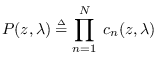
The combined probability density and discrete probability function

$$p({\bf z}) = p(y_1, \;y_2 \ldots y_{M-1} ,\; r, \; k_1, \;k_2 \ldots k_{M-1})$$

is defined as the limit as $\delta \rightarrow 0$ of $\delta^{-M}$ times the probability that the largest RV had index $k_1$ and is between $y_1-\delta/2$ and $y_1+\delta/2$, AND the next largest RV had index $k_2$ and is between $y_2-\delta/2$ and $y_2+\delta/2$, etc, AND the sum of the remaining RVs is between $r-\delta/2$ and $r+\delta/2$. The exact solution is given by [52]

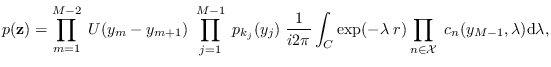$$p({\bf z}) = \prod_{m=1}^{M-2} \; U(y_m - y_{m+1} ) \; \prod_{j=1... ...(-\lambda \; r ) \prod_{n\in{\cal X}} \; c_{n}(y_{M-1},\lambda) {\rm d}\lambda,$$ (8.5)

where ${\cal X}$ is the set of indexes between $1$ and $N$ that do not include $k_1$ through $k_{M-1}$, $U(x)$ is the unit step function, $C$ is the contour in the MGF domain $\lambda$, and

$$P(z,\lambda)\stackrel{\mbox{\tiny $\Delta$}}{=} \prod_{n=1}^{N} \; c_n(z,\lambda)$$

where

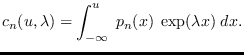$$c_n(u,\lambda)=\int_{-\infty}^u \; p_n(x) \; \exp(\lambda x) \; dx.$$ (8.6)

The best numerical solution is obtained by finding the saddlepoint (the real value of $\lambda$ for which the integrand achieves the minimum value), then integrating from $-\infty$ to $\infty$ vertically in the complex plane at that real value of $\lambda$. A saddlepoint approximation to this integral is also available [53].