Features
Let
![${\bf x}=[x_1 x_2 \ldots x_N]$](img778.png) be a set of
be a set of  independent random variables (RVs) distributed
under hypothesis
independent random variables (RVs) distributed
under hypothesis  according to the common PDF
  .
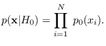
The joint probability density function (PDF)
of
.
The joint probability density function (PDF)
of  is
is
Now let  be ordered in decreasing order into the set
![${\bf y}=[y_1, y_2 \ldots y_N]$](img781.png) where
where
 .
We now choose a set of
.
We now choose a set of  indexes
 , with
 to form a selected collection of
order statistics
to form a selected collection of
order statistics
 . To this set,
we add the residual “energy",
. To this set,
we add the residual “energy",
 |
(8.1) |
where the set  are the integers from
  to
not including the values
to
not including the values
 ,
and
,
and  is a function which is needed to insure
that
is a function which is needed to insure
that  has units of energy and controls
the energy statistic.
We then form the complete feature vector of length
has units of energy and controls
the energy statistic.
We then form the complete feature vector of length  (
( ):
):
By appending the residual energy to the feature vector,
we insure that  contains the energy statistic.
We consider two important cases:
contains the energy statistic.
We consider two important cases:
- if is positive intensity
or spectral data and has approximate chi-square statistics
(resulting from sums of squares of Gaussian RV),
then
 is sufficient.
The resulting energy statistic and reference hypotheses
are the “Exponential" in Table 3.1.
For this case, we consider to be a set of magnitude-squared DFT bin outputs,
which are exponentially distributed.
is sufficient.
The resulting energy statistic and reference hypotheses
are the “Exponential" in Table 3.1.
For this case, we consider to be a set of magnitude-squared DFT bin outputs,
which are exponentially distributed.
- if are raw measurements and have
approximate Gaussian statistics,
use
 or
or
 .
The resulting energy statistic and reference hypotheses
are the “Gaussian" in Table 3.1.
For this case, we let be a set of absolute values of
zero-mean Gaussian RVs. Then, .
.
The resulting energy statistic and reference hypotheses
are the “Gaussian" in Table 3.1.
For this case, we let be a set of absolute values of
zero-mean Gaussian RVs. Then, .