The DAF integral.
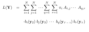
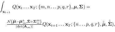
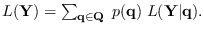
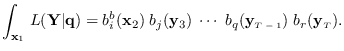
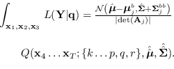
The desired integral is
 |
(15.2) |
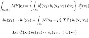
We first expand
 where
where  is a particular length-
 Markov state sequence
 with apriori probability
In what follows, the indexes
 will always stand for the assumed states at times
 ,
respectively.
Using conditional independence,
,
respectively.
Using conditional independence,
 |
(15.3) |
Thus, we have
For tractability, we assume the state observation PDFs
 are Gaussian.
This assumption does not limit this discussion since
an HMM with Gaussian mixture state PDFs can be represented as an HMM with Gaussian state PDFs
by expanding the individual mixture kernels as separate Markov states.
We assume a special form for the means and covariances
of
:
are Gaussian.
This assumption does not limit this discussion since
an HMM with Gaussian mixture state PDFs can be represented as an HMM with Gaussian state PDFs
by expanding the individual mixture kernels as separate Markov states.
We assume a special form for the means and covariances
of
:
 ![$\displaystyle _k = \left[ \begin{array}{l} \mbox{\boldmath$\mu$}_k^a \mbo...
...Sigma}_k^{ab} {\bf\Sigma}_k^{ba} & {\bf\Sigma}_k^{bb} \end{array}\right],$](img1767.png) |
(15.4) |
where superscripts  and
and  refer to
the partitions of
refer to
the partitions of  corresponding to
 and
and
 , respectively (thus, , are in order of
increasing time).
Note that the marginal PDFs are easily found,
for example
, respectively (thus, , are in order of
increasing time).
Note that the marginal PDFs are easily found,
for example
 has mean

 and covariance

The only term in (15.3) that depends on  is
is
 ,
which integrated over is
,
which integrated over is
so
 |
(15.5) |
We now proceed to integrate (15.5) over  .
The only terms that depend on are
.
The only terms that depend on are
 and
and
 .
We have
.
We have
 |
(15.6) |
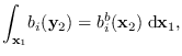
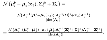
Using (15.4) and standard identities for the conditional
distribution,
,
where
and
.
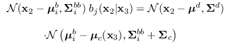
Then, using the standard identity for the product of two Gaussians,
where
Integrating over leaves us with
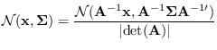
We can convert this into a density of  using the fact that for any invertible matrix
  ,
,
 |
(15.7) |
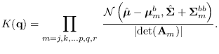
Define
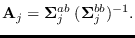 We have
So we have
 |
(15.8) |
where
 |
(15.9) |
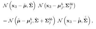
We now proceed to integrate over .
We re-write the product
 as
as
where
![\begin{displaymath}\begin{array}{l}
\hat{\hat{{\bf\Sigma}}}=\left[ \hat{{\bf\Sig...
...ma}_j^{bb})^{-1} \mbox{\boldmath$\mu$}_j^b \right].
\end{array}\end{displaymath}](img1799.png) |
(15.10) |
Collecting results and integrating over ,
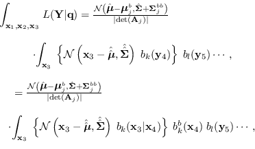 |
(15.11) |
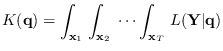
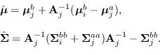
Define
then we may re-write (15.6) and (15.11) as
and
 |
(15.12) |
Comparing the above equations, we can see a recursion.
Because we have previously identified indexes
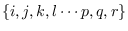 with fixed time indexes, to make a general expression
for the recursion, we need to define the free indexes
with fixed time indexes, to make a general expression
for the recursion, we need to define the free indexes
 representing the assumed Markov states
at the arbitrary times
representing the assumed Markov states
at the arbitrary times  ,
, , respectively.
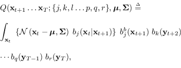
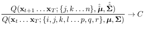
The recursion is
, respectively.
The recursion is
where
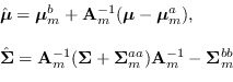 |
(15.13) |
and
![\begin{displaymath}\begin{array}{l}
\hat{\hat{{\bf\Sigma}}}=\left[ \hat{{\bf\Sig...
...ma}_m^{bb})^{-1} \mbox{\boldmath$\mu$}_m^b \right].
\end{array}\end{displaymath}](img1810.png) |
(15.14) |
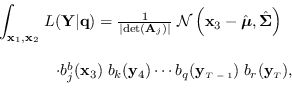
The recursion starts by integrating (15.12)
over  and ends with

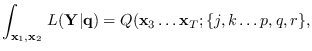
 It can be seen that the full integral
is obtained by the product
 |
(15.15) |
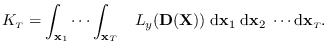
Finally, the desired integral (15.2) is given by
 |
(15.16) |
Since there are  elements in
 ,
the computation is of order
,
the computation is of order  , but the terms in
(15.15) converge to a limiting
distribution, since the ratio
, but the terms in
(15.15) converge to a limiting
distribution, since the ratio
quickly converges to
a constant  . This convergence is related
to the property of limiting distributions for Markov chains [79]
and is fortunate because
. This convergence is related
to the property of limiting distributions for Markov chains [79]
and is fortunate because
 needs only be calculated for a few values of , then the
constant stored.
needs only be calculated for a few values of , then the
constant stored.
We tested the expression for
 by comparing to the numerically-integrated PDF.
We created samples of
by comparing to the numerically-integrated PDF.
We created samples of  by selecting the first
  MFCC coeffients extracted from
some arbitrary samples of speech data and trained
an HMM on samples of
MFCC coeffients extracted from
some arbitrary samples of speech data and trained
an HMM on samples of  . With HMM parameters
held fixed, we evaluated
. With HMM parameters
held fixed, we evaluated
 using the forward procedure
on a fine grid spanning the
using the forward procedure
on a fine grid spanning the  -dimensional space of .
In theory the integral equals 1.0 for
-dimensional space of .
In theory the integral equals 1.0 for
 since in this case, and are equivalent.
For
since in this case, and are equivalent.
For  , we were able to carry out the numerical integration
up to
, we were able to carry out the numerical integration
up to  . For
. For  , the numerical integration could be carried out only up to
  .
Table 15.1 shows the comparison of
with
numerical integration as a function of .
Note the close agreement with
from equation (15.16).
The accuracy was limited by the grid sampling used in the numerical
integration since it greatly affected the computation time.
The ratio
.
Table 15.1 shows the comparison of
with
numerical integration as a function of .
Note the close agreement with
from equation (15.16).
The accuracy was limited by the grid sampling used in the numerical
integration since it greatly affected the computation time.
The ratio
 is shown to converge
quite rapidly. Therefore the values
can be extrapolated to much higher
with no additional calculations.
is shown to converge
quite rapidly. Therefore the values
can be extrapolated to much higher
with no additional calculations.
Table:
Comparison of numerically integrated likelihood function
with equation (15.16) over feature dimension
and length . The number of Markov states was  .
.
|
|
Numerical result |
|
|
| 1 |
2 |
0.999999 |
1.000000 |
1 |
| 1 |
3 |
0.412523 |
0.412307 |
0.412307 |
| 1 |
4 |
0.191555 |
0.191275 |
0.463914 |
| 1 |
5 |
0.092301 |
0.092048 |
0.481233 |
| 1 |
6 |
|
0.044915 |
0.487951 |
| 1 |
7 |
|
0.022039 |
0.490682 |
| 1 |
8 |
|
0.010839 |
0.491809 |
| 1 |
9 |
|
0.005335 |
0.492204 |
| 1 |
10 |
|
0.002628 |
0.492442 |
| 1 |
11 |
|
0.001294 |
0.492506 |
| 1 |
12 |
|
0.000637 |
0.492526 |
| 1 |
13 |
|
0.000314 |
0.492529 |
| 2 |
2 |
0.99999 |
1.000000 |
1 |
| 2 |
3 |
0.06426 |
0.063756 |
|
|