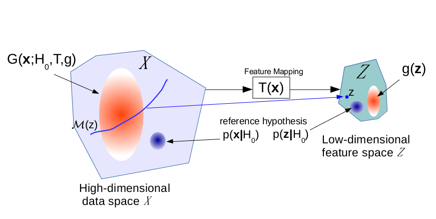
Illustration of PDF Projection

PDF projection is illustrated in Figure 2.1. In the figure, we see a feature transformation $T({\bf x})$ that maps the high-dimensional data space $\mathbb{X}$ into a lower-dimensional feature space $\mathbb{Z}$. A reference distribution $p({\bf x}\vert H_0)$ is shown in the input data space $\mathbb{X}$ and feature space $\mathbb{Z}$, where it is written $p({\bf z}\vert H_0)$. A feature distribution $g({\bf z})$ is also shown. On the basis of knowing $T({\bf x})$, $p({\bf z}\vert H_0)$, $p({\bf x}\vert H_0)$, and $g({\bf z})$, we construct the density $G({\bf x};H_0,T,g)$, using formula (2.2) which is shown in the figure. We say that $g({\bf z})$ has been projected to the input data space. Because $G({\bf x}; T, g, H_0)$ is a member of the class of distributions on $\mathbb{X}$ that generate feature distribution $g({\bf z})$ through transformation $T({\bf x})$, it is an estimate of a distribution of ${\bf x}$ that could have generated $g({\bf z})$. If $g({\bf z})$ is an estimate of the feature distribution, then $G({\bf x}; T, g, H_0)$ can be seen as an estimate of the input data distribution $p({\bf x})$.

Also seen in the figure is the level set ${\cal M}({\bf z})$, which is the set of all points ${\bf x}$ that map to a given point ${\bf z}$ in the feature space. To draw a sample from $G({\bf x};H_0,T,g)$, we first draw a sample ${\bf z}$ from $g({\bf z})$, then draw a sample from set ${\cal M}({\bf z})$. The sample is drawn from ${\cal M}({\bf z})$, not uniformly, but proportional to $p({\bf x}\vert H_0)$.

In Chapter 3, we will discuss maximum entropy PDF projection in which we choose $H_0$ to produce the distribution that has maximum entropy among all possible PDFs consistent with $g({\bf z})$. But for now, assume that $H_0$ is user-selected.

Figure 2.1: Illustration of PDF projection.